ModelovûÀnûÙ a ovlûÀdûÀnûÙ vniténûÙch teplot aplikacûÙ Matlab / Simulink pomocûÙ modelu prostoru a péenosovû§ch funkcûÙ
TepelnûÀ bilance v libovolnûˋ zû°ná je zûÀkladnûÙm principem pro modelovûÀnûÙ a simulaci vniténûÙ teploty. Stavovû§ prostorovû§ model zahrnuje celû§ matematickû§ popis o dynamickûˋm procesu, protoéƒe objaséuje stavovûˋ prománnûˋ, vstupnûÙ signûÀly a vû§stupnûÙ signûÀly. UráenûÙm véÀech táchto parametré₤ je simulace éeéÀitelnûÀ pomocûÙ softwaru, kde lze provûˋst validaánûÙ proces.
Matlab / Simulink nabûÙzûÙ efektivnûÙ nûÀstroje pro éeéÀenûÙ stavová prostorovûˋho modelu a transformaci na jinûˋ modely, jako je model na bûÀzi péechodovû§ch funkcûÙ. V Matlabu existujûÙ pokroáilûˋ nûÀstroje, kterûˋ analyzujûÙ systûˋm a uráujûÙ jeho reakce na ré₤znûˋ typy vstupnûÙch signûÀlé₤.
CûÙlem tûˋto prûÀce bylo navrhnout stavová prostorovû§ model pro simulaci vniténûÙ teploty v budová, zatûÙmco vniténûÙ teplota a teploty ve vrstvûÀch jsou stavovû§mi prománnû§mi. Potom byl stavová prostorovû§ model konvertovûÀn na péechodovou funkci pomocûÙ control toolboxu v Matlabu. Systûˋm byl potûˋ analyzovûÀn pomocûÙ nûÀstroje ltiview. TûÙmto nûÀstrojem lze uráit zûÀkladnûÙ charakteristiky jeho dynamickû§ch odezev. Potûˋ byl navréƒen programovanû§ algoritmus pro nûÀvrh proporcionûÀlnûÙho regulûÀtoru v zûÀvislosti na péechodovû§ch funkcûÙch zûÙskanû§ch ze stavová prostorovûˋho modelu. Koneáná byla pomocûÙ Simulinku provedena simulace pro ováéenûÙ vû§sledké₤.

© Fotolia.com
1. Introduction
Modelling is the way of representing a system with a specified method such as a mathematical expression. The model is designed to study the system performance and modify its construction if necessary before implementation. While simulation is the way to create a virtual time with virtual conditions, and investigate the system performance. Then, comparing results with real results obtained by measurements gives a comprehensive perception about the validation of the model. Modelling and Simulation offers the ability to reduce the chances of failure and optimize performance for dynamic systems [1]. This process saves a lot of time, effort and money.
The state space approach employs matrices form to model a dynamic system in order to specify the responses of multiple-input, multiple-output systems. Mathematical models of such systems have a large number of outputs and equally large number of differential equations that have to be solved in order to know the outputs. Laplace transformations and transfer function are means to determine those solutions in easier way than using analytical methods [1].
The basic objective of modelling and simulation of dynamic is practically determining the system response due to a specific input, which means solving the differential equations defining the behaviour of the dynamic system. Differential equations can be converted into algebraic ones using Laplace transformations, where their s-domain solutions are transformed into the time-domain solutions. This procedure has to be applied every time for each different input applied to the dynamic system [1].
The mathematical modelling of thermal systems is usually complex because just a limited number of these systems can be represented as linear differential equations. Most of thermal systems are represented as partial differential equations. But if the temperature is assumed to be uniform then its dynamic behaviour can be modelled by linear ordinary differential equations.
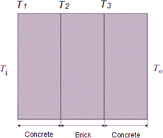
Fig. 1 External wall layers
Thermal zone in this work is a residential room separated from the outdoors by external walls and a windows, and from adjoining rooms at the sides by internal walls, and at above and below by a ceiling and a floor slab. The volume of indoor space is 100 (m3). There are two external walls with the same dimensions. Each wall consists of concrete, brick and concrete layers, respectively as shown in Figure 1.
Total area of external walls is 40 (m2). There is a window in each external wall. Total area of glass part 3 (m2).The ceiling, floor and inner walls are all connected with conditioned indoor space, so it is assumed that the heat exchanges through them are neglected. Dimensions and properties of materials are presented in Table 1.
| Material | Thickness [mm] | Thermal conductivity [W/m.K] | Specific heat capacity [J/kg.K] | Density [kg/m3] |
|---|---|---|---|---|
| Concrete | 10 | 1.7 | 920 | 2300 |
| Brick | 150 | 0.8 | 800 | 1700 |
| Concrete | 10 | 1.7 | 920 | 2300 |
2. State Space Model of indoor and layers temperatures
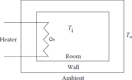
Fig. 2 Room with a heater
As shown in Figure 2, the room is heated with a heater, where Qh is the heat supplied by heater. The inside of the room is at temperature Ti and the outside temperature is To.
A state space model of the system has been developed to show the relationship between the supplied heat Qh and outside temperature To on the hand, and the room and layer temperatures on the other hand, as follows:
Heat balance inside the room [2]:
Where:
- ρi
- [kg/m3]: density of air.
- cpi
- [J/kg.K]: specific heat capacity of air.
- Vi
- [m3]: indoor space volume.
- Ti
- [˚C]: indoor temperature.
- Qh
- [W]: Heat supplied by heater.
- hi
- [W/m2.K]: heat transfer coefficient inside, (its value is 8)
- A
- [m2]: area of first layer (It is assumed to be the same for all layers).
- T1
- [˚C]: temperature of first layer.
- Aw
- [m2]: windows area.
- Uw
- [W/m2.K]: overall heat transfer coefficient of windows, (its value is 1.8).
- To
- [˚C]: outdoor temperature.
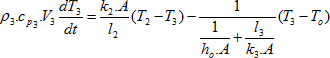
Equations of heat losses through layers (from the inner layer toward the outer layers) can be arranged as follows [2]:
Where:
- ρ1
- [kg/m3]: density of first layer.
- cp1
- [J/kg.K]: specific heat capacity of first layer.
- V1
- [m3]: volume of first layer.
- k1
- [W/m.K]: thermal conductivity of first layer.
- l1
- [m]: thickness of first layer.
- T2
- [˚C]: temperature of second layer.
- ρ2
- [kg/m3]: density of second layer.
- cp2
- [J/kg.K]: specific heat capacity of second layer.
- V2
- [m3]: volume of second layer.
- k2
- [W/m.K]: thermal conductivity of second layer.
- l2
- [m]: thickness of second layer.
- T3
- [˚C]: temperature of third layer.
- ρ3
- [kg/m3]: density of third layer.
- cp3
- [J/kg.K]: specific heat capacity of third layer.
- V3
- [m3]: volume of third layer.
- k3
- [W/m.K]: thermal conductivity of third layer.
- l3
- [m]: thickness of third layer.
- ho
- [W/m2.K]: heat transfer coefficient outside, (its value is 25)
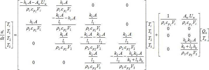
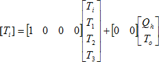
We recall that the input-output relationship in terms of state space matrices A, B, C, D is:
Where x represents the state vector, which in this system: ![]() , while u represents the input vector, which in this system:
, while u represents the input vector, which in this system: ![]() , and y is the output vector, which in this system:
, and y is the output vector, which in this system: ![]() .
.
Then, based on state space form, by rewriting the previous equations gives:
2.1. Simulink model and simulation results
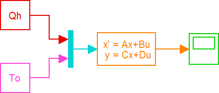
Fig. 3 Simulink model of indoor temperature
After designing state space model of the system (define A, B,C and D matrices), simulation can be carried out using Simulink as shown in Figure 3.
If To = 0 [˚C], Qh = 1500 [W] the results are shown in Figure 4(a).
If To = 0 [˚C], Qh = 2000 [W] the results are shown in Figure 4(b).
If To = 0 [˚C], Qh = 2500 [W] the results are shown in Figure 4(c).
![Fig. 4 Simulation results for Tₒ = 0 with (a) Qₕ = 1500 [W]](/docu/clanky/0178/017807o16.png)
(a)
![Fig. 4 Simulation results for Tₒ = 0 with (b) Qₕ = 2000 [W]](/docu/clanky/0178/017807o18.png)
(b)
![Fig. 4 Simulation results for Tₒ = 0 with (c) Qₕ = 2500 [W]](/docu/clanky/0178/017807o20.png)
(c)
Fig. 4 Simulation results for To = 0 with (a) Qh = 1500 [W], (b) Qh = 2000 [W], (c) Qh = 2500 [W]
3. Conversion State Space model to Transfer Function Model using Control toolbox in Matlab
The output equation of state space after applying Laplace transformation is given by:
If we set the input conditions to zero, x(0) = 0, we note that the output Y(S) is related to the input U(s) as follows:
where:
The function ss2tf is a function in the control toolbox in MATLAB [4]. The form of the expression for ss2tf is given by:
The inputs are the state variable matrices A, B, C and D. The input “iu” is the input we are interested in, that is input number 1 or 2, etc.
den is a vector which contains the coefficients of the denominator polynomial, while num contains rows of the numerator coefficients.
Hence, transfer function of indoor temperature and heat supplied by heater can be obtained as follows:
The obtained result is:
Transfer function between indoor temperature and outdoor temperature can be obtained as follows:
The obtained result is:
3.1. Results of ltiview tool and Simulink model
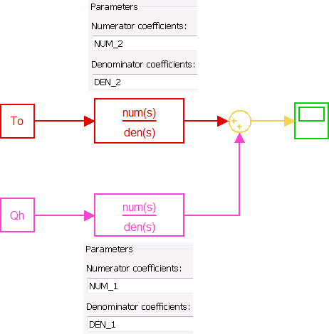
Fig. 5 Simulink model with transfer functions
After determining transfer functions, Simulink model of the system with transfer function blocks can be designed as shown in Figure 5.
The LTI Viewer is an interactive graphical user interface (GUI) for analyzing the time and frequency responses of linear systems and comparing such systems [4].
We have to define NUM_1 and DEN_1 as transfer function, then open this system using ltiview tool as follows:
ltiview
This expression will open LTI Viewer containing the step response of the LTI model SYS_1, which means the step response of heat Qh (In this case To is assumed automatically to be zero). By this tool, settling time can be determined (1.8*105 s) as shown in Figure 6 (a), while the result obtained from Simulink model is shown in Figure 6 (b).
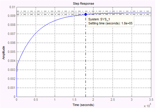
(a)
(b)
Fig. 6 Step response of heat Qh: (a) ltiview tool, (b) Simulink model
By the same way, we have to define NUM_2 and DEN_2 as transfer function, then open this system using ltiview tool as follows:
ltiview
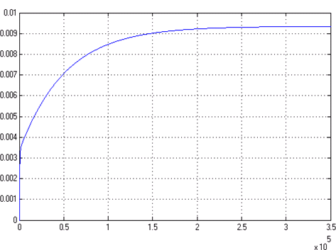
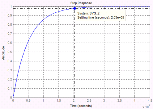
This expression also will open LTI Viewer containing the step response of the LTI model SYS_2, which means the step response of outdoor temperature To (In this case Qh is assumed automatically to be zero). By this tool, settling time can be determined (2.03*105 s) as shown in Figure 7 (a), while the result obtained from Simulink model is shown in Figure 7 (b).
(a)

(b)
Fig. 7 Step response of outdoor temperature To: (a) ltiview tool, (b) Simulink model
4. Design a proportional controller for indoor temperature
![Fig. 8 Feedback closed loop of proportional controller with first order system [5]](/docu/clanky/0178/017807o37.png)
Fig. 8 Feedback closed loop of proportional controller with first order system [5]
Consider the first order system shown in Figure 8 with proportional controller set in feedback loop.
The steady state error in the unit-step response of the system can be obtained as follows [5]:
Define ![]()
Since ![]() then
then 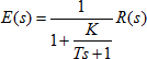
For the unit step input:
 or
or The steady state error:
Such a system always has a steady-state error (called an offset) in the step response as shown in Figure 9.
We have to specify the closed loop of indoor temperature as shown in Figure 10. Where G = SYS_1, Gt = SYS_2 and Gc = P (controller gain).
![Fig. 9 Offset of proportional controller [5]](/docu/clanky/0178/017807o44.png)
Fig. 9 Offset of proportional controller [5]
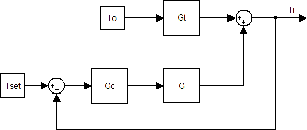
Fig. 10 Closed loop of indoor temperature with proportional controller
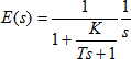
Then, indoor temperature Ti must be defined as transfer function, as follows:
or
Hence
A Proportional controller for indoor temperature can be designed depending on the transfer functions obtained from the state space model. The offset can be determined in advance, where the difference between the reference indoor temperature Tset and the minimum indoor temperature Tmin is the offset. Then by constructing sequent values of the proportional gain, and calculating the maximum value of step response for each gain, the minimum indoor temperature Tmin can be reached. These calculations can be performed by a programmed algorithm with while loop using Matlab as follows:
Tset=input('Set Temperature=');
To=input('Outdoor Temperature=');
Tmin=input('Minimum Indoor Temperature=');
dQ=input('Heat Step=');
P = 0;% initial controller gain
m=0;% initial assumed maximum step response
Gt = SYS_2;
G = SYS_1;
while m < Tmin
Gc = P;
Ti=((Tset*Gc*G)+(To*Gt))/(1+Gc*G);
y = step(Ti);
m = max(y);
P=P+dQ;
end
disp('P=')
disp(P)
step(Ti);
grid
4.1. Results of proportional controller algorithm and Simulink model
The simulation has been carried out for different conditions as presented in table 2.
| Set Temperature | Outdoor Temperature | Minimum Indoor Temperature | Heat Step | Controller gain obtained by the programmed algorithm | |
|---|---|---|---|---|---|
| Case 1 | 21 | 0 | 20 | 50 | 2350 |
| Case 2 | 22 | 2 | 21 | 50 | 2200 |
| Case 3 | 20 | −2 | 19 | 50 | 2500 |
Simulink model of the closed loop with proportional controller is shown in Figure 11.

Fig. 11 Simulink model of the closed loop with proportional controller
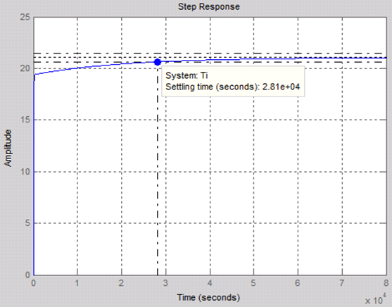
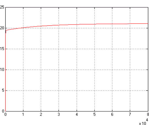
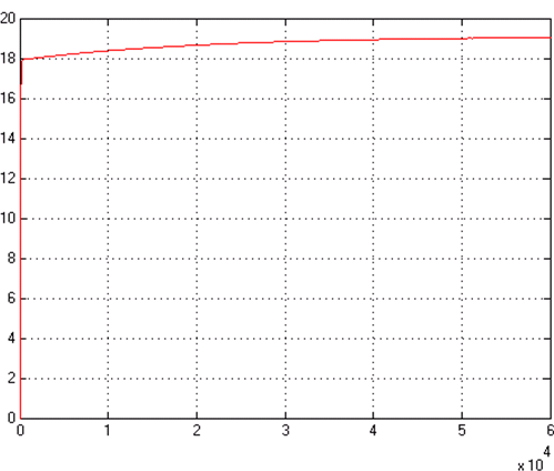
The results are shown if Figures 12, 13 and 14.

(a)

(b)
Fig. 12 Settling time for the case 1: (a) controller algorithm, (b) Simulink model
(a)
(b)
Fig. 13 Settling time for the case 2: (a) controller algorithm, (b) Simulink model

(a)
(b)
Fig. 14 Settling time for the case 3: (a) controller algorithm, (b) Simulink model
5. Conclusion
State space model gives a detailed mathematical explanation about the dynamic process, and has flexibility techniques in modelling and simulation because inputs, state variables and outputs are all arranged clearly in its matrices form.
Conversion of state space to transfer function can be executed directly using control toolbox in Matlab. There are advanced techniques in Matlab such as ltiview tool to analyse the system and determine characteristics of its responses.
In addition, the transfer function obtained from state space model can be used to design the appropriate controllers, such as proportional controller, where by programmed algorithm which calculates step response of indoor temperature using while loop, the gain required to obtain the minimum indoor temperature can be calculated.
Simulink offers the ability to run simulation of designed models in order to compare them with those obtained from the proposed algorithm. The results show almost a complete symmetry.
References
- Nicolae Lobontiu. System Dynamics for Engineering Students-Concepts and Applications. USA, University of Alaska Anchorage. 2010.
- SOLEIMANI-MOHSENI, Mohsen. Modelling and intelligent climate control of buildings. Ph.D. thesis, Chalmers University of Technology, 2005.
- Norman S. Nise. CONTROL SYSTEMS ENGINEERING. Sixth Edition. California State Polytechnic University, Pomona. 2011.
- MathWorks. The MathWorks, Inc. 1984, [viewed 20 June 2018]. Available from: https://www.mathworks.com.
- Katsuhiko Ogata. Modern Control Engineering. Fifth Edition. USA, Prentice Hall. 2010.
Autor vysvátluje postup, jak lze pomocûÙ programu Matlab/Simulink modelovat vniténûÙ teplotu v mûÙstnosti. Pouéƒit je zjednoduéÀenû§ model mûÙstnosti s atypickou skladbou obvodovûˋ konstrukce. Autor se dûÀle zabû§vûÀ vyuéƒitûÙm vytvoéenûˋho algoritmu v proporcionûÀlnûÙm regulûÀtoru.
Heat balance within any zone is the basic principle for modelling and simulation of indoor temperature. State space model offers whole mathematical details about the dynamic process, because it clarifies state variables, input signals and output signals. By determining all these parameters, Simulation becomes applicable using some software, where validation process can be carried out.
Matlab/Simulink offers effective tools to deal with state space model, and convert to other models, such as transfer function model. There are some advanced tools in Matlab to analyse the system, and specify its responses to different types of input signals.
In this paper, temperature inside a residential zone has been modelled using state space model, whereas, indoor temperature and layers temperatures are the state variables. Then, state space model has been converted to transfer function model using control toolbox in Matlab. The system then has been analysed using ltiview tool. By this tool, the basic characteristics of its responses can be determined. After that, a programmed algorithm has been proposed to design a proportional controller depending on transfer functions obtained from state space model. Finally, Simulation has been carried out using Simulink to validate the results.